Implicit Regularization in RL Post-Training

RLHF pipelines employ a variety of explicit regularization techniques to prevent over-optimization of the reward model. The most common is a KL divergence penalty from a reference model, first applied to sequence generation by Jaques et al. (2017). Ouyang et al. (2022) added pretraining gradients, an auxiliary next-token-prediction loss on a held-out corpus to maintain general language ability. Pang et al. (2024) introduced NLL anchoring in DPO, a length-normalized log-likelihood term on winning completions to keep preferred outputs high-probability in an absolute sense. Touvron et al. (2023) proposed margin-based losses for reward models, injecting annotator confidence scores as explicit margins between chosen and rejected pairs.

A growing body of empirical work reveals that RL-based post-training also provides implicit regularization — a built-in resistance to memorization and catastrophic forgetting that emerges from the structure of on-policy optimization itself, even without any explicit KL penalty or replay buffer.

SFT Memorizes, RL Generalizes

A core question facing the post-training community has been: When training on a single task, does the model learn a generalizable rule that transfers to unseen variants, or does it memorize the surface patterns of the training distribution? Chu et al. (2025) answer this question with a controlled empirical study that directly isolates the effect of the post-training method — SFT versus RL — on out-of-distribution (OOD) generalization. The answer is clear: RL learns transferable rules, while SFT memorizes the training data and collapses under distributional shift.

The study uses two environments with built-in rule variations:

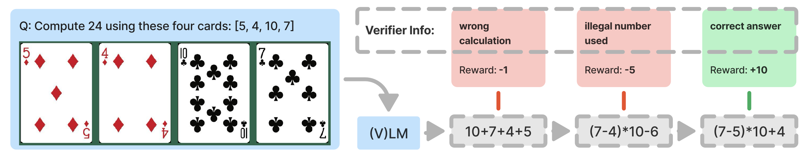
GeneralPoints is an arithmetic card game where the model receives four playing cards and must combine their numerical values with operators (+, -, *, /) to reach a target number (24 by default). The OOD test changes how face cards are scored: training uses one rule (Jack, Queen, and King all count as 10), evaluation uses another (Jack = 11, Queen = 12, King = 13).
V-IRL is a real-world visual navigation task where models follow linguistic instructions to traverse a route through city streets, recognizing landmarks along the way. The OOD shift switches the action space from absolute directions (north, east) to relative directions (left, right).

Across all task variants, RL consistently improves OOD performance as training compute scales up, while SFT consistently degrades OOD performance despite improving in-distribution. The magnitude of divergence is striking: on V-IRL with language-only inputs, where the OOD shift is from absolute to relative directional coordinates, RL improves OOD per-step accuracy from 80.8% to 91.8%, while SFT collapses from 80.8% to 1.3%. The SFT model goes further than failing to generalize: it destroys the spatial reasoning the base model already had, collapsing to a lookup table from instruction phrases to absolute directions.

SFT memorizes while RL generalizes across distributional shifts — RL consistently improves out-of-distribution performance as training progresses, while SFT degrades it despite improving in-distribution. From Chu et al. 2025.

Retaining by Doing: On-Policy Data Mitigates Forgetting

The previous section showed that RL generalizes where SFT memorizes on a single task. Chen et al. (2025) ask the complementary question: when training sequentially on multiple tasks, does the model retain what it already knew? They find that RL achieves comparable or higher gains on target tasks while forgetting substantially less than SFT, and trace this advantage to a fundamental difference in what the two objectives optimize.

To understand why the two methods behave so differently, we can view their objectives through the lens of KL divergence, which can be expressed in two directions:

Forward KL: $\text{KL}(P \| Q) = \mathbb{E}_{x \sim P}[\log P(x) - \log Q(x)]$
Reverse KL: $\text{KL}(Q \| P) = \mathbb{E}_{x \sim Q}[\log Q(x) - \log P(x)]$

where $P$ is the target distribution and $Q$ is the distribution we are modeling with parameters $\theta$. The key difference is which distribution we sample from: forward KL samples from the target (or optimal) distribution $P$, whereas reverse KL samples from our policy $Q$. In the derivations below, $P$ corresponds to the target $\pi_\star$ (the training data distribution when analyzing SFT, or the reward-optimal policy when analyzing RL) and $Q$ to the learned policy $\pi_\theta$. SFT places the target first — $\text{KL}(\pi_\star \| \pi_\theta)$ — while RL flips the order — $\text{KL}(\pi_\theta \| \pi_\star)$ — changing which distribution we sample from.

SFT ≈ Forward KL. Let $\pi_\star$ be the target distribution for our dataset. Then, the forward KL divergence is:

$$ \begin{aligned} \text{KL}(\pi_\star \| \pi_\theta) &= \mathbb{E}_{(x,y) \sim \mathcal{D}} \left[ \log \pi_\star(y \mid x) - \log \pi_\theta(y \mid x) \right] \\ &= \mathbb{E}_{(x,y) \sim \mathcal{D}} \left[ \log \pi_\star(y \mid x) \right] - \mathbb{E}_{(x,y) \sim \mathcal{D}} \left[ \log \pi_\theta(y \mid x) \right] \\ &= \underbrace{-H(\pi_\star)}_\text{const} + \mathcal{L}_\text{SFT}(\theta) \\ &\propto \mathcal{L}_\text{SFT}(\theta) \end{aligned} $$

Since $H(\pi_\star)$ is constant with respect to $\theta$, minimizing the SFT loss is exactly equivalent to minimizing the forward KL divergence $\text{KL}(\pi_\star \| \pi_\theta)$.

RL ≈ Reverse KL. Let us start with the standard KL-regularized RL objective:

$$ \max_\pi \; \mathcal{J}_\text{RL}(\theta) = \mathbb{E}_{x \sim \mathcal{D},\, y \sim \pi(\cdot \mid x)} \left[ r(x, y) \right] - \beta \cdot \text{KL}\!\left(\pi(\cdot \mid x) \| \pi_\text{ref}(\cdot \mid x)\right) $$

Pulling out $-\beta$ converts maximization to minimization:

$$ = \min_\pi \; \mathbb{E}_{x \sim \mathcal{D},\, y \sim \pi(\cdot \mid x)} \left[ \log \frac{\pi(y \mid x)}{\pi_\text{ref}(y \mid x)} - \frac{1}{\beta} r(x, y) \right] $$

Introducing a partition function $Z(x) = \sum_y \pi_\text{ref}(y \mid x) \exp\!\left(\frac{1}{\beta} r(x,y)\right)$ to normalize the reward-tilted reference into a valid distribution, and adding and subtracting $\log Z(x)$, the inner expectation becomes a KL divergence:

$$ = \min_\pi \; \mathbb{E}_{x \sim \mathcal{D}} \left[ \text{KL}\!\left(\pi(\cdot \mid x) \;\middle\|\; \frac{1}{Z(x)} \pi_\text{ref}(\cdot \mid x) \exp\!\left(\tfrac{1}{\beta} r(x,y)\right) \right) - \log Z(x) \right] $$

Since $\log Z(x)$ does not depend on $\pi$, the KL is minimized at zero when $\pi$ equals the reward-tilted distribution. The optimal policy under reward $r(x,y)$ is therefore:

$$ \pi_\star(y \mid x) = \frac{1}{Z(x)} \pi_\text{ref}(y \mid x) \exp\!\left(\frac{1}{\beta} r(x,y)\right) $$

Now we can show the connection to reverse KL directly. Expanding $\text{KL}(\pi_\theta \| \pi_\star)$ and substituting $\log \pi_\star(y \mid x) = \log \pi_\text{ref}(y \mid x) - \log Z(x) + \frac{1}{\beta} r(x, y)$:

$$ \begin{aligned} \text{KL}(\pi_\theta \| \pi_\star) &= \mathbb{E}_{x \sim \mathcal{D},\, y \sim \pi_\theta(\cdot \mid x)} \left[ \log \pi_\theta(y \mid x) - \log \pi_\star(y \mid x) \right] \\ &= \mathbb{E}_{x \sim \mathcal{D},\, y \sim \pi_\theta(\cdot \mid x)} \left[ \log \pi_\theta(y \mid x) - \log \pi_\text{ref}(y \mid x) + \log Z(x) - \frac{1}{\beta} r(x, y) \right] \\ &= - \frac{1}{\beta} \mathbb{E}_{x,y}\!\left[r(x,y)\right] + \text{KL}\!\left(\pi_\theta(\cdot \mid x) \;\middle\|\; \pi_\text{ref}(\cdot \mid x)\right) + \underbrace{\log Z(x)}_\text{const} \\ &\propto - \frac{1}{\beta} \mathbb{E}_{x,y}\!\left[r(x,y)\right] + \text{KL}\!\left(\pi_\theta(\cdot \mid x) \;\middle\|\; \pi_\text{ref}(\cdot \mid x)\right) \\ &= -\frac{1}{\beta} \mathcal{J}_\text{RL}(\theta) \end{aligned} $$

Equivalently, maximizing the RL objective $\mathcal{J}_\text{RL}(\theta)$ is the same as minimizing the reverse KL divergence $\text{KL}(\pi_\theta \| \pi_\star)$.

This derivation shows that SFT and RL optimize fundamentally different objectives: SFT minimizes forward KL, RL minimizes reverse KL.

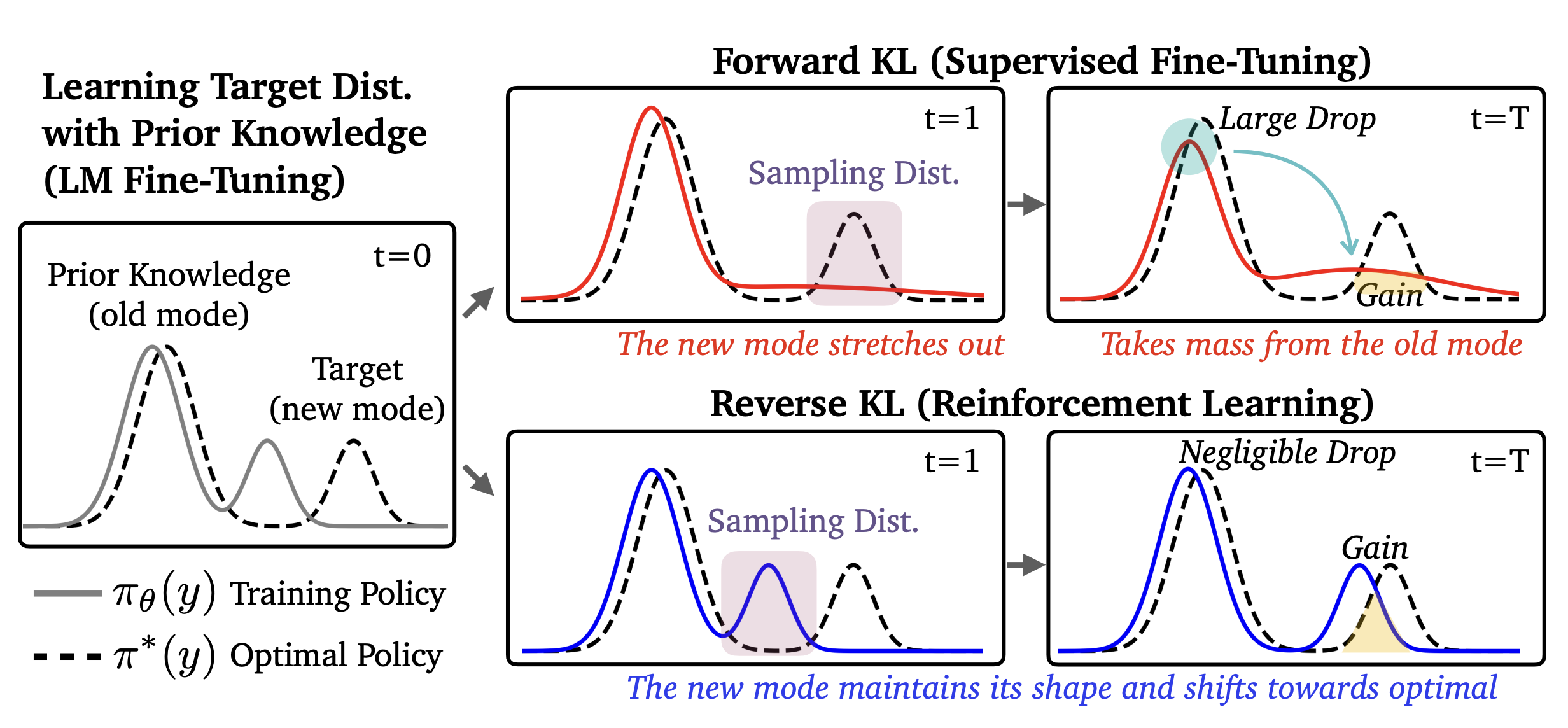
Forgetting dynamics for forward KL (SFT) versus reverse KL (RL). The "old" mode represents prior knowledge, the "new" mode represents the target task. Forward KL stretches the policy to cover the target and pulls mass away from the old mode (top right), while reverse KL shifts the new mode toward the target without disturbing the old mode (bottom right). From Chen et al. 2025.

Forward KL penalizes the model whenever the target distribution has mass where the model does not, which forces the model to cover all modes of the target — spreading probability broadly even if it means assigning mass to low-probability regions (mode covering). Reverse KL only penalizes the model in regions where it actually places mass, which allows it to seek a single mode and fit it precisely while ignoring others entirely (mode seeking).

Given this distinction, we might naively expect SFT to forget less than RL: mode-covering forward KL should maintain mass across all modes of the target, preserving old knowledge, while mode-seeking reverse KL could collapse onto a single high-reward mode and abandon others.

However, the opposite holds. This intuition assumes a unimodal policy, but pre-trained LLMs contain multiple modes — and for multimodal distributions, the dynamics flip.

Consider a policy with two modes: an "old" mode representing prior knowledge and a "new" mode for the target task (see the figure above). Forward KL (SFT) must cover both modes of the target distribution, which forces the policy to stretch and redistribute probability mass from the old mode, disrupting its shape and causing forgetting. Reverse KL (RL), by contrast, only needs to place mass on some high-reward region, so it can shift the new mode toward the target without touching the old mode at all, leaving prior knowledge intact.

RL's mode-seeking behavior — a structural property of reverse KL — preserves the breadth of the model's prior knowledge and enables better generalization.

To summarize:

SFT (Forward KL): $\text{KL}(\pi_\star \| \pi_\theta)$ — samples come from the target $\pi_\star$, a fixed dataset of human-written completions. For each example, we ask: how much probability does our model $\pi_\theta$ assign to this? The model never generates anything; it learns to imitate. This mode-covering pressure forces the policy to redistribute mass broadly, which can disrupt prior knowledge.
RL (Reverse KL): $\text{KL}(\pi_\theta \| \pi_\star)$ — samples come from our own policy $\pi_\theta$. For each completion the model generates, we ask: how close is this to the reward-optimal policy $\pi_\star$? Because the model only trains on its own generations, updates stay local to where it already places probability mass — the reward signal tells it which of those generations to reinforce, shifting probability toward $\pi_\star$ without disturbing the rest of the distribution.

RL's Razor: Why Online RL Forgets Less

The previous section showed that on-policy sampling drives RL's forgetting resistance and traced the mechanism to forward-vs-reverse KL dynamics. Shenfeld, Pari, and Agrawal (2026) offer a complementary perspective, again through the lens of KL divergence.

For any given task, there exist many distinct policies which achieve high performance. Shenfeld, Pari, and Agrawal (2026) introduce the RL's Razor thesis which postulates the following:

Among the many high-reward solutions for a new task, on-policy methods such as RL are inherently biased toward solutions that remain closer to the original policy in KL divergence.

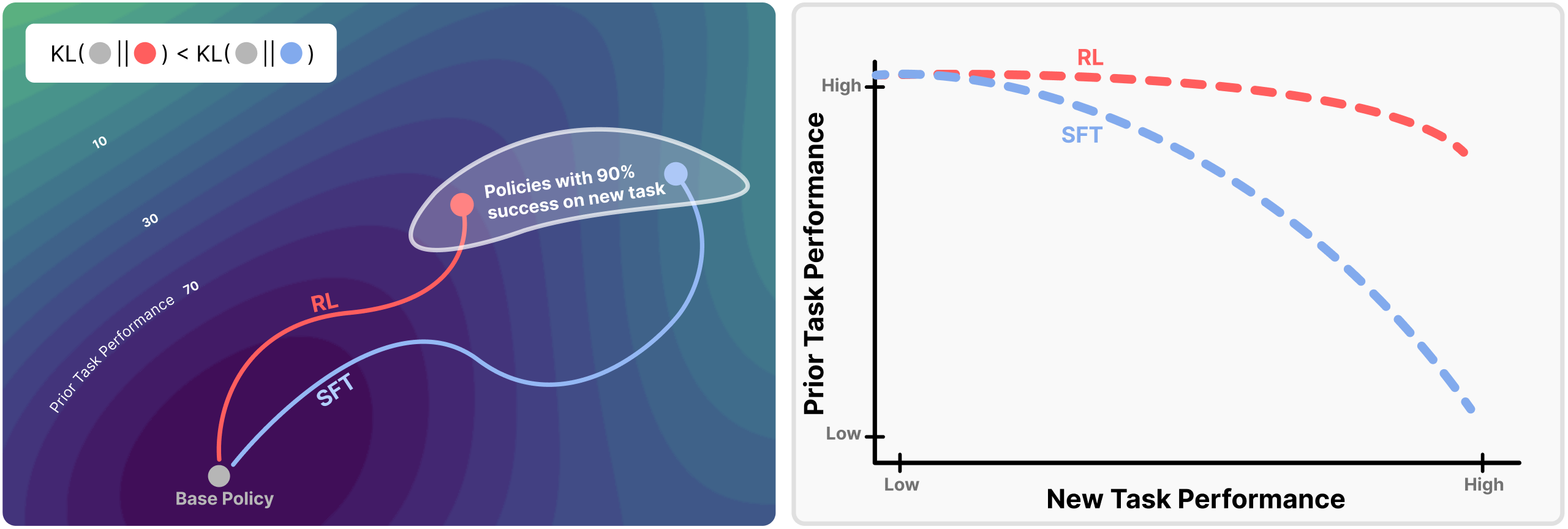
Bias toward KL-minimal solutions reduces forgetting. (Left) Among policies that solve the new task, RL converges to those closest in KL to the base model. (Right) This KL bias yields higher prior-task retention at matched new-task performance compared to SFT. From Shenfeld, Pari, and Agrawal 2026.

The authors find that forgetting of past tasks is directly proportional to how far the fine-tuned policy drifts from the initial model as measured by the KL divergence:

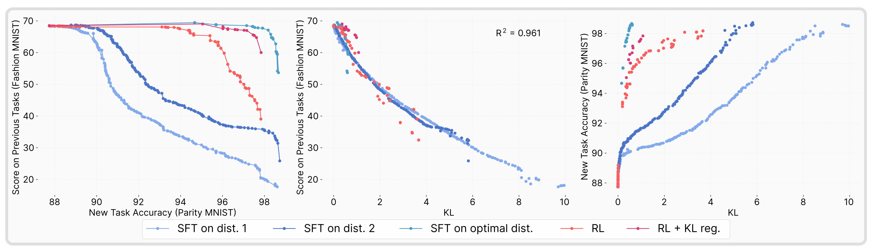
$$ \text{Forgetting} \approx f\!\left(\mathbb{E}_{x \sim \tau}\!\left[\text{KL}\!\left(\pi_0(\cdot \mid x) \| \pi(\cdot \mid x)\right)\right]\right) $$

Across several training flavors of RL and SFT, the authors empirically demonstrate that forgetting strongly correlates ($R^2 = 0.96$) with the KL divergence between the trained and initial policies, as measured using the new task data. The result is highly non-trivial: the KL is measured on the new task's input distribution, not on held-out data from prior tasks, yet it still predicts the performance drop on past tasks. In practice, this provides us with a powerful instrument for estimating forgetting directly from the drift between the base and trained policies.

Forgetting correlates with KL divergence from the base policy — Forgetting strongly correlates ($R^2 = 0.96$) with the KL divergence between the trained and initial policies, measured on new-task data. From Shenfeld, Pari, and Agrawal 2026.

To pin down what drives the smaller KL shifts in RL policies, the authors decompose the difference between RL and SFT along two axes — on-policy versus offline data, and whether the objective includes negative gradients (present in RL when samples score below the reward baseline, absent in SFT which only reinforces correct demonstrations) that push probability away from incorrect outputs. Remarkably, they find that on-policy versus offline data fully accounts for the difference in generalization performance, while negative gradients have no discernible effect.

Perhaps most strikingly, the authors also show that performing SFT on an optimal oracle distribution — one that achieves the lowest KL divergence from the base policy among all high-performing policies — yields the best overall performance while retaining substantially more prior knowledge than standard SFT. This result suggests that the forgetting problem is not inherent to SFT's learning mechanism per se, but rather to the mismatch between the fixed training distribution and the model's own distribution. When the training data is explicitly constructed to stay close to the base policy in KL space, SFT can match RL's retention properties, reinforcing the thesis that the KL distance from the base model is the key predictor of forgetting regardless of the training method.

Intuitively, on-policy methods sample outputs the model already assigns non-negligible probability to, so each update is constrained to stay near the current distribution. On the other hand, SFT trains on a fixed external distribution that can lie arbitrarily far from what the model currently produces, and each gradient step pulls toward that distant target regardless of the model's own beliefs.