Confident Learning

Real-world datasets are noisy. Once you look closely at the labels in widely-used benchmarks like ImageNet, MNIST, or Amazon Reviews, three problems keep showing up:

• Plain mistakes. A handwritten 4 labeled 9 in MNIST.
• Hierarchical overlap. ImageNet has separate classes for missile and projectile, but every missile is a projectile. The paper finds 645 ImageNet images labeled missile that look more like the parent class. The two labels are not mutually exclusive, yet the dataset treats them as if they were.
• Inherently multilabel content. A single ImageNet image with both a chain-link fence and a military uniform has to get one label. Whichever the annotator picked, the other is technically wrong, but neither label is.

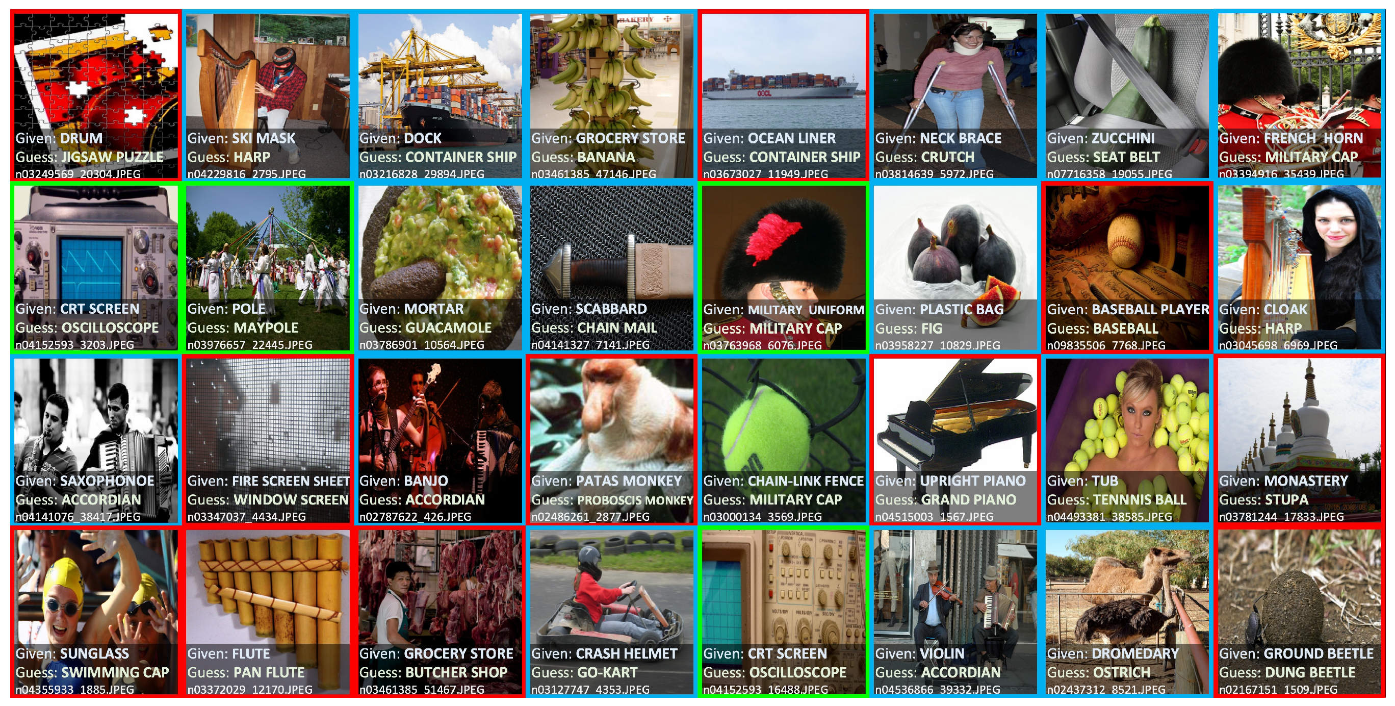
In this post we will work through the framework that produced the figure above: Confident Learning (CL). Given a trained classifier's out-of-sample predicted probabilities and the dataset's noisy labels, CL estimates the joint distribution of noisy and true labels directly, then uses that joint to find, rank, and prune mislabeled examples, without retraining or relabeling.

The Pipeline

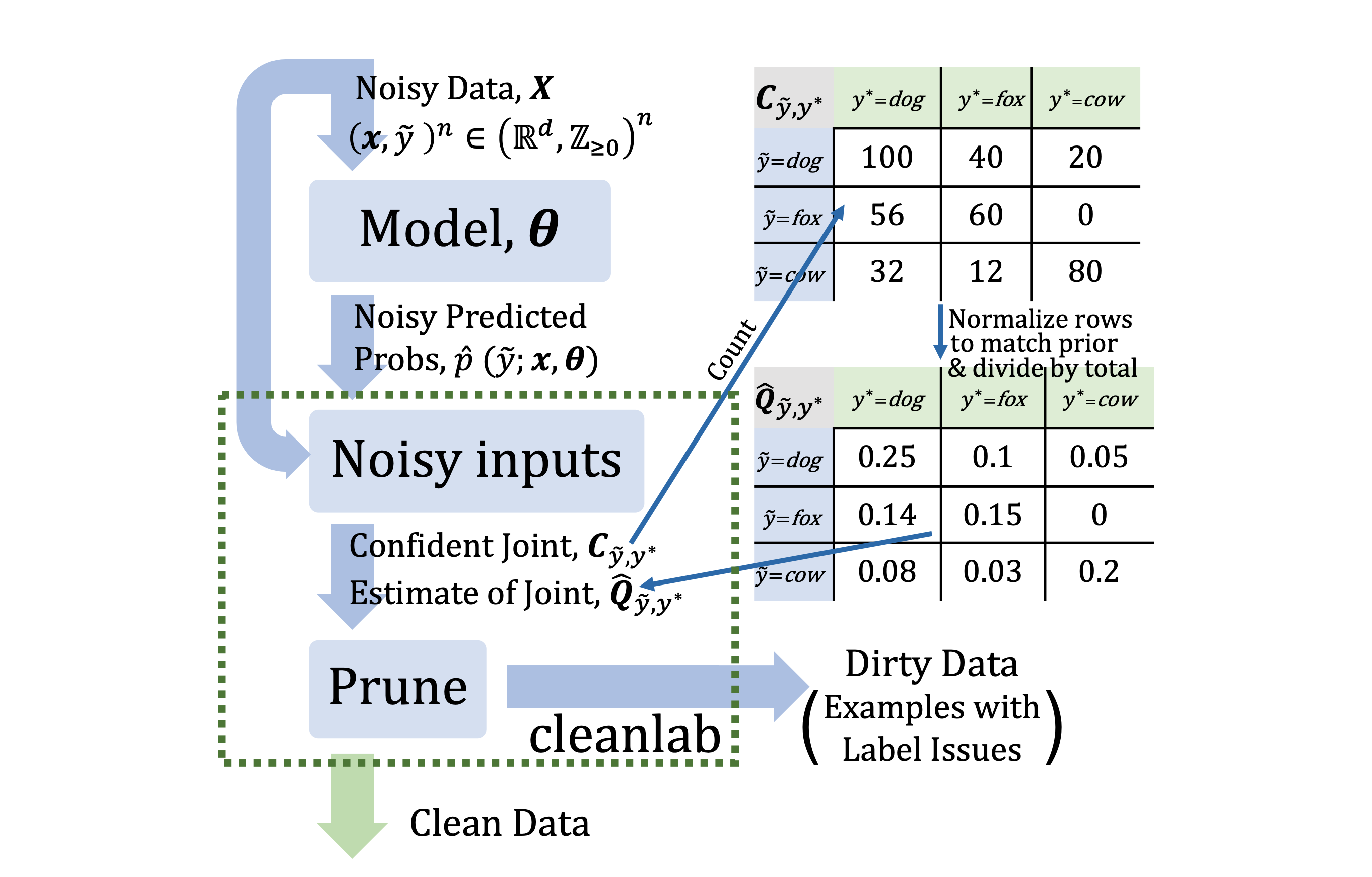
We start with a dataset of \(n\) samples with noisy labels, \(\mathcal{D} = (x, \tilde y)^n\), where each \(x \in \mathbb{R}^d\) carries an observed class label \(\tilde y \in \{1, \ldots, m\}\) that may be wrong. We train a classifier on \(\mathcal{D}\) using \(k\)-fold cross-validation, which produces an out-of-sample predicted probability \(\hat P_{k,i} \coloneqq \hat p(\tilde y = i \mid x_k, \theta)\) for every sample \(x_k\) and every class \(i \in \{1, \ldots, m\}\).

The Confident Joint

The central object is the confident joint \(C_{\tilde y, y^*}\), an \(m \times m\) matrix of counts where \(C[i][j]\) is the number of examples currently labeled \(i\) that "confidently belong" to class \(j\). \(C[i{=}3][j{=}1] = 10\) reads: ten examples are labeled 3 but should be labeled 1.

What does "confidently belong" mean? The naive option is to take the argmax of the predicted probabilities. The problem is that probabilities are heterogeneous across classes: one class might be systematically over-confident and win most argmaxes, while another sits low and never wins. CL avoids this with a per-class threshold:

$$ t_j = \frac{1}{|\mathcal{D}_{\tilde y = j}|} \sum_{x \in \mathcal{D}_{\tilde y = j}} \hat p(\tilde y = j \mid x, \theta) $$

\(t_j\) is the average self-confidence of the dataset's class-\(j\) examples: on average, how much probability does the model assign to class \(j\) for the examples already labeled \(j\)? An over-confident class gets a high bar; an under-confident class gets a low one – therefore, the threshold scales with the class.

An example \(x\) with noisy label \(i\) is then counted in cell \(C[i][j]\) if two conditions hold:

1. \(\hat p(\tilde y = j \mid x, \theta) \ge t_j\).
2. If more than one class clears its threshold, \(j\) is the one with the highest predicted probability (this resolves collisions, which can occur when softmax outputs are smooth enough that an example passes several thresholds at once).

Formally:

$$ \begin{aligned} C_{\tilde y, y^*}[i][j] &\coloneqq \left| \hat{\mathcal{D}}_{\tilde y = i,\, y^* = j} \right|, \\ \hat{\mathcal{D}}_{\tilde y = i,\, y^* = j} &\coloneqq \left\{ x \in \mathcal{D}_{\tilde y = i} \;:\; \hat p(\tilde y = j \mid x, \theta) \ge t_j, \;\; j = \arg\max_{l \,:\, \hat p(\tilde y = l \mid x, \theta) \ge t_l} \hat p(\tilde y = l \mid x, \theta) \right\} \end{aligned} $$

Diagonal entries \(C[i][i]\) count examples whose noisy label agrees with the model's confident guess. Off-diagonals \(C[i][j],\, i \neq j\), are the label-error counts: examples labeled \(i\) that look like \(j\). A toy example from the paper with classes \(\{\text{dog}, \text{fox}, \text{cow}\}\):

$$ C_{\tilde y, y^*} = \begin{array}{c|ccc} & y^* = \text{dog} & y^* = \text{fox} & y^* = \text{cow} \\ \hline \tilde y = \text{dog} & 100 & 40 & 20 \\ \tilde y = \text{fox} & 56 & 60 & 0 \\ \tilde y = \text{cow} & 32 & 12 & 80 \end{array} $$

The diagonal \((100, 60, 80)\) holds examples whose noisy label is supported by the model. The off-diagonals are candidate errors: 40 examples labeled dog that the model confidently calls fox, 56 labeled fox that look like dog, 32 labeled cow that look like dog, and so on.

From \(C\) to the Joint Distribution

\(C\) is an unnormalized count matrix. To turn it into an estimate \(\hat Q_{\tilde y, y^*}\) of the true joint distribution \(p(\tilde y, y^*)\), the pipeline applies two calibrations: row-calibrate so that each row sums to the observed noisy-class marginal \(|\mathcal{D}_{\tilde y = i}|\), then normalize so the whole matrix sums to 1.

$$ \hat Q_{\tilde y = i,\, y^* = j} = \frac{\dfrac{C_{\tilde y = i,\, y^* = j}}{\sum_{j' = 1}^{m} C_{\tilde y = i,\, y^* = j'}} \cdot |\mathcal{D}_{\tilde y = i}|}{\displaystyle\sum_{i' = 1}^{m} \sum_{j' = 1}^{m} \left( \frac{C_{\tilde y = i',\, y^* = j'}}{\sum_{j'' = 1}^{m} C_{\tilde y = i',\, y^* = j''}} \cdot |\mathcal{D}_{\tilde y = i'}| \right)} $$

Why row-calibrate first? \(C\) only counts examples that cleared at least one threshold, so it silently drops the ones the model wasn't confident about. The number dropped is not uniform across classes, so \(C\)'s row sums no longer match the true noisy-class counts \(|\mathcal{D}_{\tilde y = i}|\). If we skipped row-calibration and just divided by the grand total, we'd be estimating the joint over the surviving confident subset, which over-represents easy classes. Row-calibration says: trust the confident subset only for the split across true classes within row \(i\), but rescale the row back to the true count we know from the data. The noisy-class marginal is then preserved exactly, and only the conditional \(p(y^* \mid \tilde y = i)\) comes from the confident subset, where it's trustworthy.

Let's apply this to the toy \(C\) from above. Assume a balanced dataset with 200 examples per noisy class, so \(|\mathcal{D}_{\tilde y = i}| = 200\) for all \(i\) and \(n = 600\). The row sums of \(C\) are \(160, 116, 124\). Rescaling each row to 200:

$$ \tilde C = \begin{array}{c|ccc} & y^* = \text{dog} & y^* = \text{fox} & y^* = \text{cow} \\ \hline \tilde y = \text{dog} & 125.00 & 50.00 & 25.00 \\ \tilde y = \text{fox} & 96.55 & 103.45 & 0.00 \\ \tilde y = \text{cow} & 51.61 & 19.35 & 129.03 \end{array} $$

Dividing by the grand total (600) gives \(\hat Q\):

$$ \hat Q_{\tilde y, y^*} = \begin{array}{c|ccc} & y^* = \text{dog} & y^* = \text{fox} & y^* = \text{cow} \\ \hline \tilde y = \text{dog} & 0.2083 & 0.0833 & 0.0417 \\ \tilde y = \text{fox} & 0.1609 & 0.1724 & 0.0000 \\ \tilde y = \text{cow} & 0.0860 & 0.0323 & 0.2151 \end{array} $$

Finding Label Issues with cleanlab

With \(C\) and \(\hat Q\) in hand, the cleanlab library exposes the following as the main entry point:

find_label_issues(labels, pred_probs, ...)

with two core knobs that control its behavior:

• filter_by selects which examples to flag as label issues.
• return_indices_ranked_by selects how to order the flagged examples from worst to least-bad (so you can review the top-\(k\) most suspicious ones first).

1. filter_by

Decides which examples are flagged. Options:

• prune_by_noise_rate (default). For each off-diagonal cell \((i, j)\) of \(\hat Q\), the joint says we expect \(n \cdot \hat Q_{\tilde y = i,\, y^* = j}\) examples to be labeled \(i\) but really be \(j\). The filter goes into class \(i\) and removes exactly that many examples, choosing the ones with the largest margin \(\hat p(\tilde y = j \mid x) - \hat p(\tilde y = i \mid x)\). It does this for every off-diagonal cell.
• prune_by_class. Aggregates the budget per row instead of per cell: for each class \(i\), expect \(n \cdot \sum_{j \neq i} \hat Q_{\tilde y = i,\, y^* = j}\) total errors. Remove that many examples from class \(i\), choosing the ones with the lowest self-confidence \(\hat p(\tilde y = i \mid x)\). Per-class budget, ranked by how poorly the model believes the given label.
• both. Intersection: only flag examples that both prune_by_noise_rate and prune_by_class would prune. High precision, lower recall.
• confident_learning. Flag everything that landed in an off-diagonal partition \(\hat{\mathcal{D}}_{\tilde y = i,\, y^* = j},\, i \neq j\) when \(C\) was built. No ranking inside the partition: membership is the flag. This matches the confident-joint definition exactly and is what the original paper proves consistency for.

2. return_indices_ranked_by

Orders the flagged examples from worst to least-bad (lower score = more suspicious). Options:

• self_confidence (default). Score by \(\hat p(\tilde y = i \mid x)\) for the given label - lowest first.
• normalized_margin. Score by \(\hat p(\tilde y = i \mid x) - \max_{j \neq i} \hat p(\tilde y = j \mid x)\). Lowest (most negative) first.
• confidence_weighted_entropy. Combines entropy of the predicted distribution with self-confidence.

Written by Zafir Stojanovski and Claude Opus 4.7.